This blog is an ongoing assignment for Gov 1347: Election Analytics, a course at Harvard College taught by Professor Ryan Enos. It will be updated weekly and culminate in a predictive model of the 2024 presidential election.
Introduction – How competitive are presidential elections in the United States? Which states vote blue/red and how consistently?
As data analysts and political scientists get geared up for an exciting 2024 Presidential Election between Kamala Harris (Democrat) and Donald Trump (Republican), we must first understand the landscape from historical data. This will give us the context necessary to build a substantial model that will hopefully predict the winner within reasonable margins.
A Starting Point
To begin, let’s start by examining the two-party presidential popular vote over time in the US from 1948 to 2020. The following is a line plot depicting how each political party’s presidential popular vote has fluctuated over the decades indicated above.
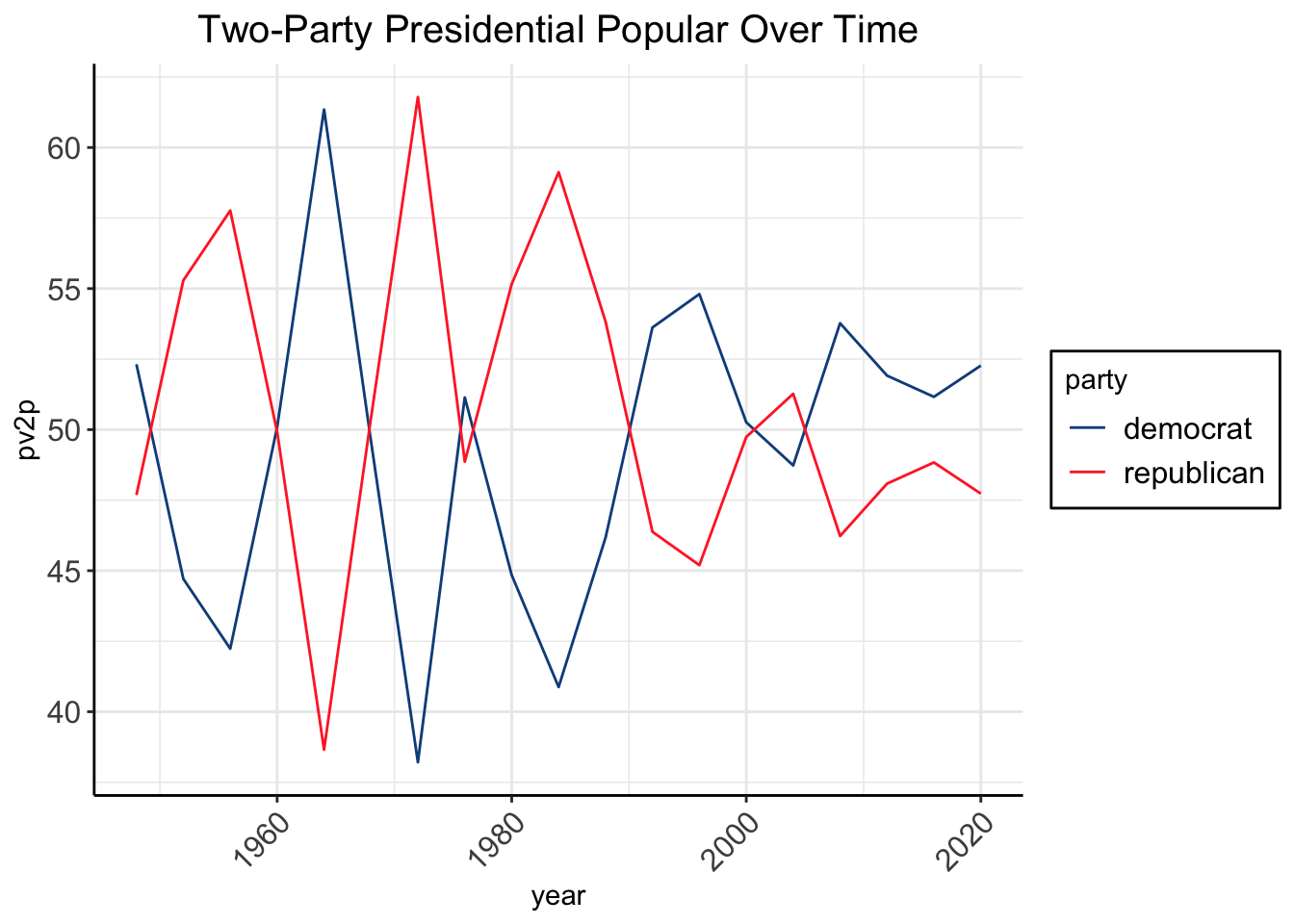
Looking at the graph above, note that the Republican vote share is the exact inverse of the Democratic vote share. This makes sense since we’re analyzing two-party vote share: Republican (R) + Democrat (D) = 1, meaning R = 1 - D. Mathematically, we can verify the visualization.
Next, we observe substantial volatility from the 1960s to the 1980s, portrayed by sharp increases and decreases by both party graph lines. Historically, this was a period of great change and turmoil in American history. For example, the Civil Rights Movement, the Vietnam War, and the Watergate scandal had dramatic influences on electoral shifts and popular vote decisions. Entering the 1990s and beyond saw periods of stability and a narrowing of political polarization. More importantly, the economy and global economic conditions played greater roles in determining voter trends. For example, in the 21st century, such as the 2004 and 2016 elections, saw an increased emphasis on economic dynamics (Fair 2018). Variables such as the growth rate of real GDP per capita, inflation, and the number of strong growth quarters played significant roles in determining voter behavior. Further analysis of economic influence will be discussed in later blog posts, so stay tuned!
Geographical Additions
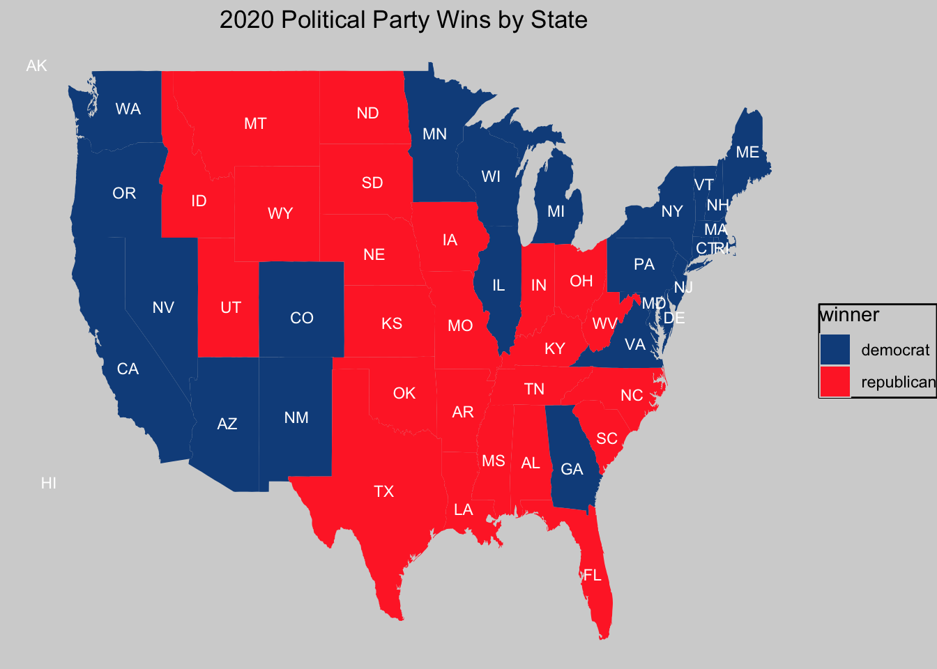
Figure 1: Added state abbreviations and custom theme as part of possible blog extension
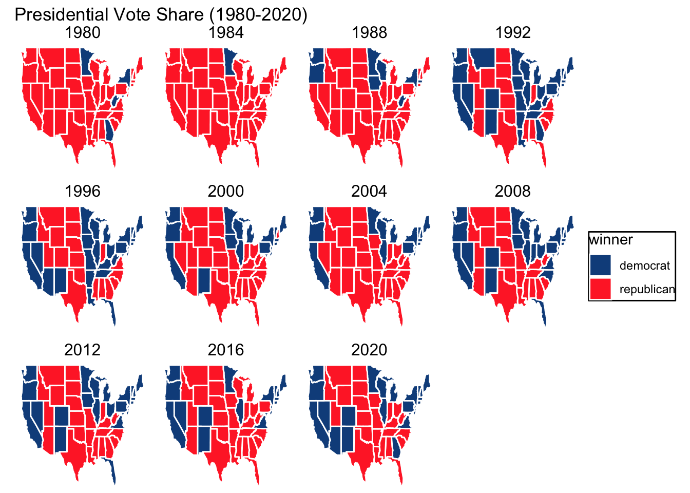
From the second visualization, we observe that some states consistently vote for one party, indicating strong partisanship and party loyalty. More specifically, western coastal states like California, Oregon, and Washington and northeastern states, such as New York and Massachusetts, have consistently voted Democratic (blue). In contrast, the south and midwest states like Texas, Oklahoma, and Alabama have stuck with Republican candidates.
Research suggests factors like demographics, geography, cultural values, and economic conditions play key roles in these consistent states. For example, states with large urban populations with greater racial and ethnic diversity historically lean left compared to more white, working-class voters in southern states. Traditionally Christian communities in Alabama, Mississippi, and Oklahoma remain stiff on social issues that align more closely with the right. These are just a few significant identifiers among these states in a larger tug-of-war between blue and red.
Interestingly, we also see clear swing states among such regional loyalty like Florida, Ohio, and Pennsylvania with far more partisan variability over time. Some battlegrounds (eg. Texas) even include many large urban centers, such as Austin and Houston, that lean left but remain overshadowed by the strength of suburban conservative voters. These will likely be key battleground areas that can shift the direction for both parties, amplifying the competitiveness of an already tense election.
A Simple Model
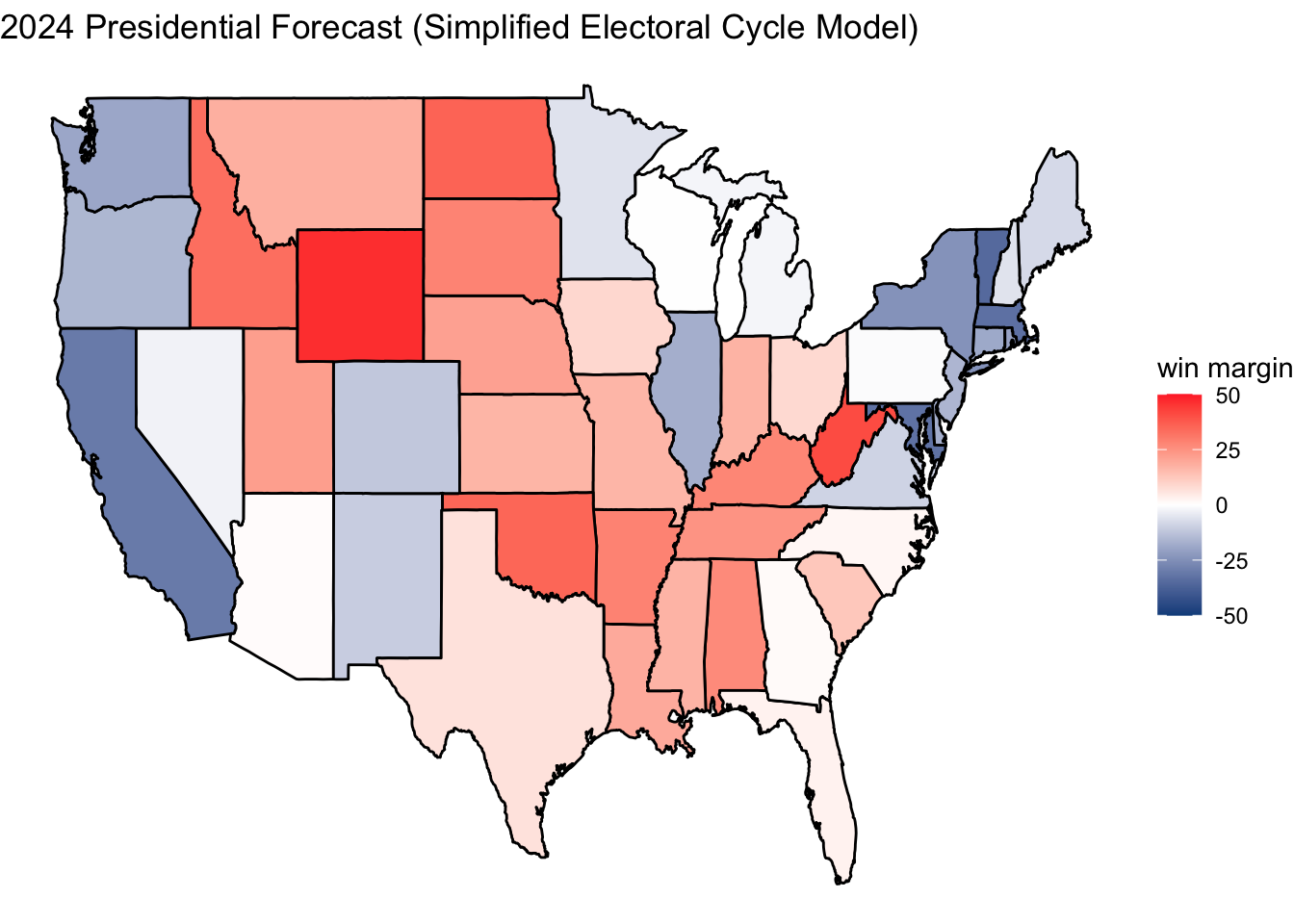
The Helmut Norpoth Primary Model uses a weight average of the two-party vote share from previous election data to predict future election results. For our purposes, we will use a simplified version of the model, weighting (3/4) with the 2020 election and (1/4) with the 2016 election. The results are shown below:
## # A tibble: 2 × 2
##   winner electoral_votes
##   <chr>            <dbl>
## 1 D                  276
## 2 R                  262
Looking at the simple forecasting model above, we can see how swing states (nearly white, meaning zero or very small win margin) continue to be up for grabs, while consistently red and blue states still show similar patterns. The model predicts Harris winning the electoral college, but southwest and sunbelt states, such as Nevada and Arizona, will continue to be contentious, particularly with shifting political attitudes and younger Latino voters (Kim 2022) becoming more involved. These changes will only heighten the competitive nature of this year’s election, making the challenge of predicting the election ever more interesting.
Now What?
Overall, we’ve understood which states vote blue/red over time and how the presidential elections remain extremely competitive with candidates vying to win over swing states, new young voters, and shifting urban demographics. With an extensive understanding of the historical two-party presidential vote share and geographic voting data, we can now begin diving deeper into more fundamental influences that shape elections, now and in the future.
Data Sources:
Data are from the GOV 1347 course materials. All files can be found here. All external sources are hyperlinked.