This blog is an ongoing assignment for Gov 1347: Election Analytics, a course at Harvard College taught by Professor Ryan Enos. It will be updated weekly and culminate in a predictive model of the 2024 presidential election.
Introduction – How can we best use polls to predict election outcomes?
What’s the first thing you hear when you flick on news channels covering any election? Polls. We’ve done hundreds of them ourselves in our lifetime, from restaurant surveys to product reviews and presidential candidates. These quick little quizzes help provide direct insights from the public about various issues, including voting behavior, candidate favorability, and more. Generally speaking, they serve as feedback loops, allowing parties and campaigns to adjust their strategies based on how the public responds during an election cycle. Breaking these statistics down by demographic categories allows these candidates to further tailor their messaging to specific audiences.
However, there are common pitfalls related to polling, including sampling bias, nonresponse bias, timing, and more. It’s our job to figure out what matters and what doesn’t. More importantly, can we use them to help predict election outcomes, or will they simply lead us astray? Let’s dive in!
2020 and 2024 Polling – A Detailed Analysis

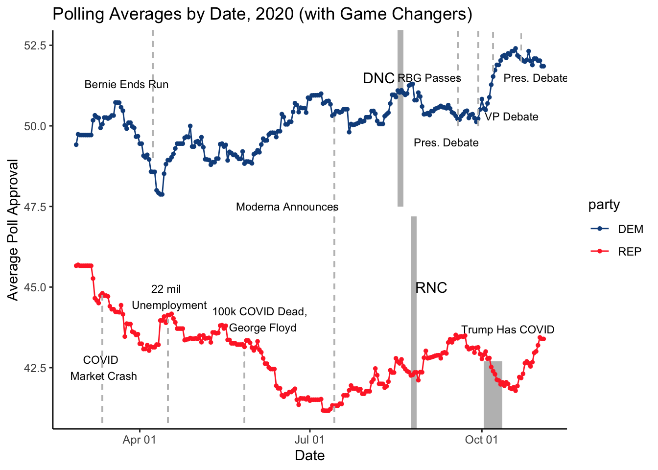
Immediately, we can notice some interesting trends. First, before COVID-19 hit, both democratic and republican polling averages were roughly stable. However, once COVID-19 was in full swing, we saw a significant decline in Republican approval, likely due to the public’s perception of how Trump was handling the pandemic, on both healthcare and economic fronts. With George Floyd’s death, we see a further decline in Republican approval, especially in handling racial injustice and social upheaval. Both the RNC and DNCs showed a bump in approval allowing parties to get in front of viewers, increase media coverage, and consolidate support.

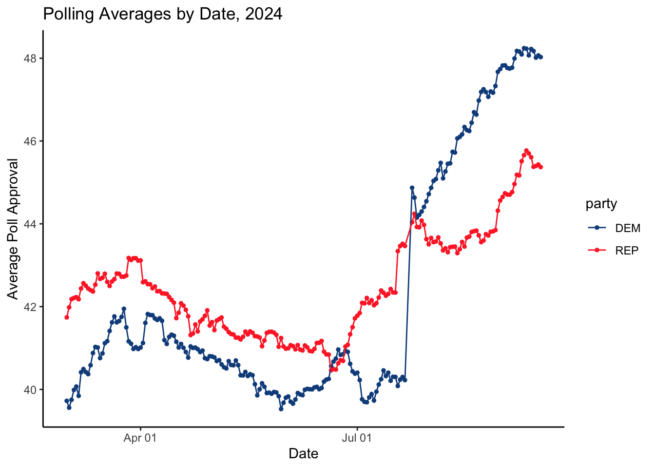
Looking at 2024 polling averages, we see a general candidate disapproval trend for both parties. Particularly for the Biden administration, the democratic party was struggling to gain ground as the November election quickly approached. The sharp increase we observed for the democrats in July has to do largely with Biden’s decision to drop out of the race and endorse Kamala Harris as the democratic presidential candidate. Moreover, her strong performance in the recent debate proved her capabilities as a leader and her vision for the future which many Americans seemed to resonate with, skyrocketing average polling approval past Trump.
Altogether, we can see the influence of major political, social, and health-related events on candidate approval, which can be captured by polling averages. Now the question is, do these polling behaviors provide any predictive power? Let’s find out!
Polls and Predictions – How about November?
Before we look into 2024, let’s examine how powerful November polling averages were at predicting election outcomes for the democratic party in 2020:
##
## Call:
## lm(formula = pv2p ~ nov_poll, data = subset(d_poll_nov, party ==
##     "DEM"))
##
## Residuals:
##     Min      1Q  Median      3Q     Max
## -4.0155 -2.4353 -0.3752  1.4026  5.8014
##
## Coefficients:
##             Estimate Std. Error t value Pr(>|t|)
## (Intercept)  14.2936     7.1693   1.994 0.069416 .
## nov_poll      0.7856     0.1608   4.885 0.000376 ***
## ---
## Signif. codes:  0 '***' 0.001 '**' 0.01 '*' 0.05 '.' 0.1 ' ' 1
##
## Residual standard error: 2.968 on 12 degrees of freedom
## Multiple R-squared:  0.6654,	Adjusted R-squared:  0.6375
## F-statistic: 23.86 on 1 and 12 DF,  p-value: 0.0003756
There are a few critical results to note about the model above. First, the coefficient for nov_poll (0.7856) means that for each 1-point increase in November polling support, the predicted vote share increases by 0.79. Moreover, the p-value is extremely small (0.000376), indicating that the nov_poll variable is a statistically significant predictor of pv2p. What’s more impressive is the multiple R-squared value of 0.66554 (closer to 1 is better), showing us that the model provides a reasonably good fit and reliability. In the context of the 2020 election results, we can see that polling support in November was a strong indicator of electoral success. Due to its proximity to election day, November polls can capture the most recent public opinion, particularly since voters will have likely made up their minds by now. As we’ve seen before, major campaign events have great influences on voter support and approval, and as the election nears, there are simply fewer of these so opinions are less volatile.
Instead of focusing solely on the democratic party, let’s widen our scope to all parties in the dataset in the following model:
##
## Call:
## lm(formula = pv2p ~ nov_poll, data = d_poll_nov)
##
## Residuals:
##     Min      1Q  Median      3Q     Max
## -4.6190 -1.6523 -0.5808  1.3629  6.0220
##
## Coefficients:
##             Estimate Std. Error t value Pr(>|t|)
## (Intercept) 17.92577    4.15543   4.314 0.000205 ***
## nov_poll     0.70787    0.09099   7.780 2.97e-08 ***
## ---
## Signif. codes:  0 '***' 0.001 '**' 0.01 '*' 0.05 '.' 0.1 ' ' 1
##
## Residual standard error: 2.75 on 26 degrees of freedom
## Multiple R-squared:  0.6995,	Adjusted R-squared:  0.6879
## F-statistic: 60.52 on 1 and 26 DF,  p-value: 2.974e-08
Similar to our previous model, we see that the nov_poll coefficient (0.70787) means that for each 1-point increase in November polling support, the predicted vote share increases by roughly 0.71 points. The positive relationship indicates that higher polling support in November is strongly associated with higher vote share. Once again, we see that the p-value is extremely low, reinforcing the statistical significance of November’s reliability as an indicator. A strong 0.7 R-squared value also provides confidence that the model is robust and captures the data effectively. More importantly, this model confirms that November polls are a strong predictor of election outcomes, regardless of party affiliation.
The Power of Weeks? Regularization Methods
Instead of looking just at November results, let’s examine how our model performs when we consider weekly polling averages. Of course, we run into an alarming issue – multicollinearity. This occurs when we have several variables in our model that are highly correlated, producing a potentially skewed view of our results. To handle this, we’ll use ridge regression, which introduces a penalty term to the least squares cost function, preventing the coefficient from becoming too large, and helping to adjust the multicollinearity factor.
Let’s examine our results:
##
## Call:
## lm(formula = paste0("pv2p ~ ", paste0("poll_weeks_left_", 0:30,
##     collapse = " + ")), data = d_poll_weeks_train)
##
## Residuals:
## ALL 28 residuals are 0: no residual degrees of freedom!
##
## Coefficients: (4 not defined because of singularities)
##                    Estimate Std. Error t value Pr(>|t|)
## (Intercept)        28.25534        NaN     NaN      NaN
## poll_weeks_left_0   3.24113        NaN     NaN      NaN
## poll_weeks_left_1   0.02516        NaN     NaN      NaN
## poll_weeks_left_2  -8.87360        NaN     NaN      NaN
## poll_weeks_left_3   7.91455        NaN     NaN      NaN
## poll_weeks_left_4   0.74573        NaN     NaN      NaN
## poll_weeks_left_5   1.41567        NaN     NaN      NaN
## poll_weeks_left_6  -4.58444        NaN     NaN      NaN
## poll_weeks_left_7   4.63361        NaN     NaN      NaN
## poll_weeks_left_8  -0.95121        NaN     NaN      NaN
## poll_weeks_left_9  -1.55307        NaN     NaN      NaN
## poll_weeks_left_10 -1.38062        NaN     NaN      NaN
## poll_weeks_left_11  1.74881        NaN     NaN      NaN
## poll_weeks_left_12 -1.28871        NaN     NaN      NaN
## poll_weeks_left_13 -0.08482        NaN     NaN      NaN
## poll_weeks_left_14  0.87498        NaN     NaN      NaN
## poll_weeks_left_15 -0.16310        NaN     NaN      NaN
## poll_weeks_left_16 -0.34501        NaN     NaN      NaN
## poll_weeks_left_17 -0.38689        NaN     NaN      NaN
## poll_weeks_left_18 -0.06281        NaN     NaN      NaN
## poll_weeks_left_19 -0.17204        NaN     NaN      NaN
## poll_weeks_left_20  1.52230        NaN     NaN      NaN
## poll_weeks_left_21 -0.72487        NaN     NaN      NaN
## poll_weeks_left_22 -2.76531        NaN     NaN      NaN
## poll_weeks_left_23  4.90361        NaN     NaN      NaN
## poll_weeks_left_24 -2.04431        NaN     NaN      NaN
## poll_weeks_left_25 -0.76078        NaN     NaN      NaN
## poll_weeks_left_26 -0.47860        NaN     NaN      NaN
## poll_weeks_left_27       NA         NA      NA       NA
## poll_weeks_left_28       NA         NA      NA       NA
## poll_weeks_left_29       NA         NA      NA       NA
## poll_weeks_left_30       NA         NA      NA       NA
##
## Residual standard error: NaN on 0 degrees of freedom
## Multiple R-squared:      1,	Adjusted R-squared:    NaN
## F-statistic:   NaN on 27 and 0 DF,  p-value: NA
The model shows that we have no residual degrees of freedom, meaning we have perfect multicollinearity, which happens when there is an exact linear dependence among the predictors – in this case, weekly polling averages. The R-squared value is 1.0, indicating a perfect fit, but this is misleading since this fit is not due to the model’s inherent capabilities, but rather from overfitting caused by too many correlated predictors.
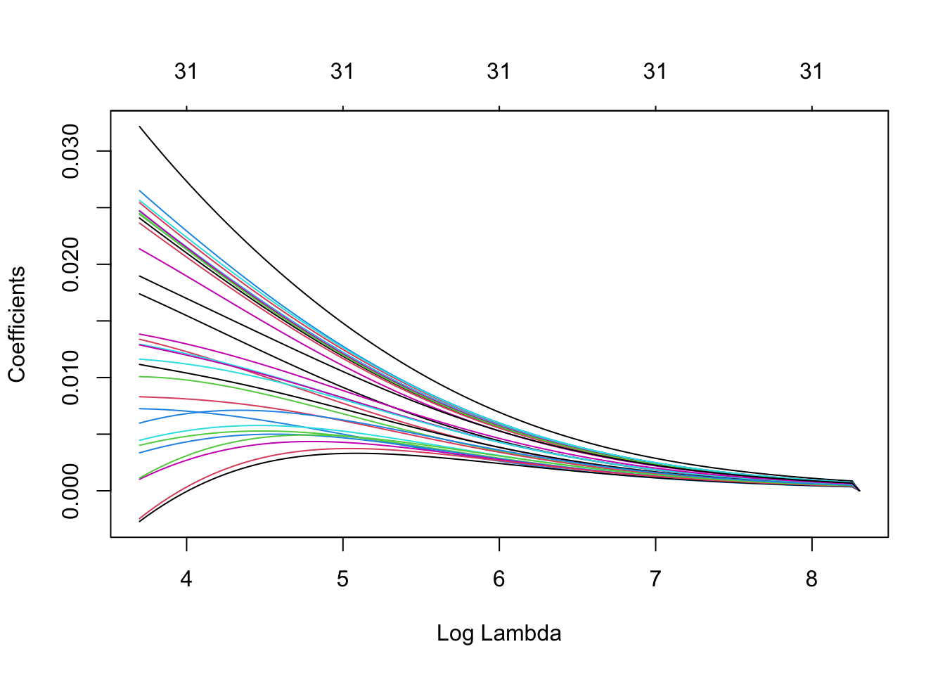
To better understand what we’re doing, let’s visualize our ridge regression:

We can clearly see lambda acting as the regularization parameter here, adding more penalty to the coefficients and shrinking them towards zero to fight the multicollinearity and overfitting. This prevents any single variable from dominating the model, which is particularly important when dealing with models containing lots of correlated variables. Of course, there are many other regularization methods, including Lasso and Elastic Net, each with its own attributes.
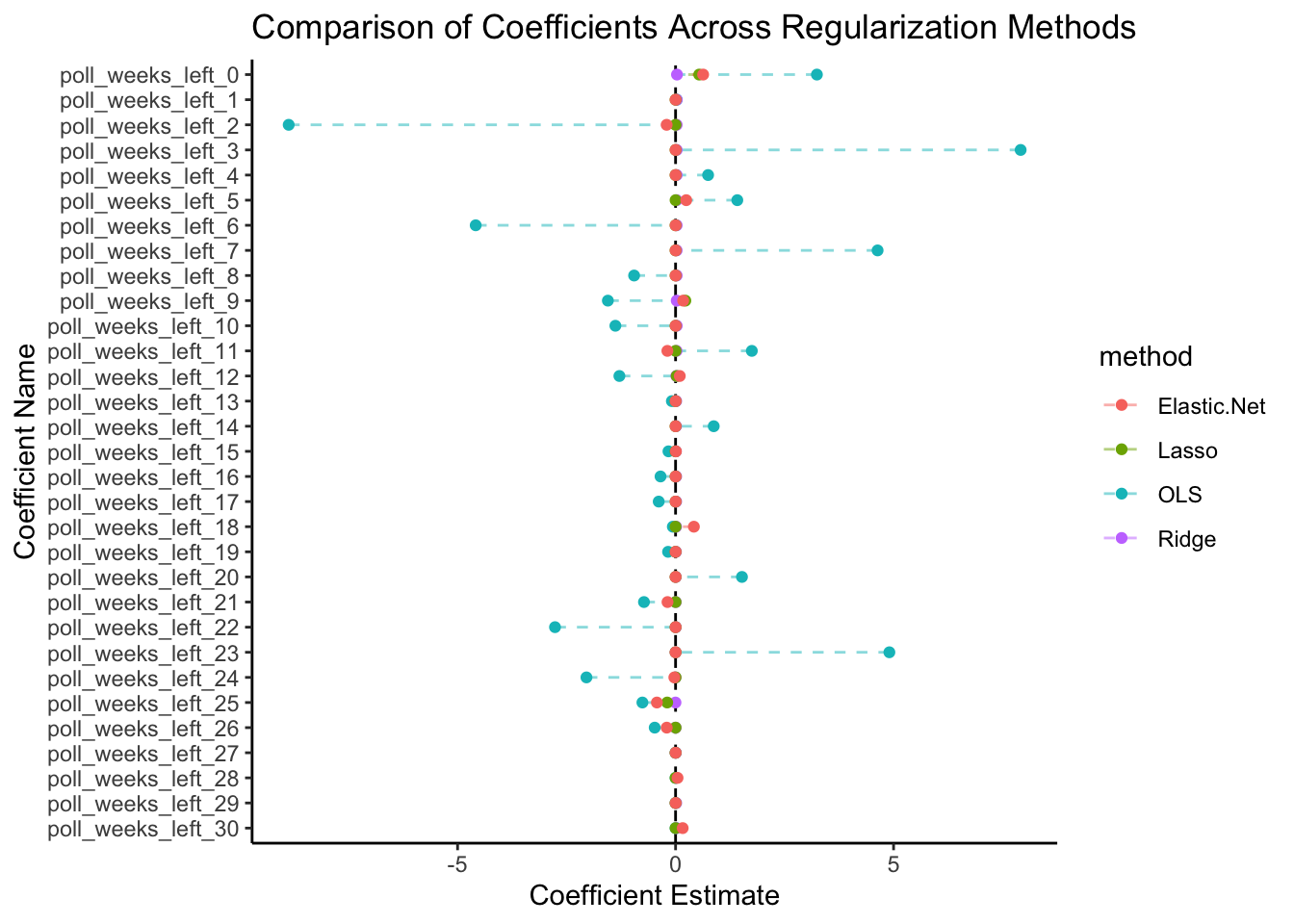
For the purposes of this blog, we will dive straight into a comparison between all three and draw conclusions, instead of an in-depth examination of each method:

By visualizing the four methods above, we see how OLS coefficients are larger compared to the regularized methods, which suggests strong overfitting, particularly in the presence of multicollinearity. Lasso and Ridge perform reasonably well, but Elastic Net performs the best, striking a balance between model complexity and highlighting key predictor variables.
Now that we have our chosen method, let’s what the model tells us about the 2024 election results:
##            s1
## [1,] 51.79268
## [2,] 50.65879
Our current polling model predicts that Harris will win the results indicate that Harris will win the vote share by a very slim margin. Assuming that our historical data is representative of current dynamics and changes to voting behavior, the Elastic-net method helps handle multicollinearity and provides a balance between shrinkage and variable elimination. Further sensitivity testing should be used to get a better understanding of the reliability of its predictions.
A Battle of Two Pollsters
To extend our knowledge of polling, let’s take a look at two different approaches. Silver’s methodology takes on a more conservative approach, by keeping his model largely unchanged from 2020, with a few specific updates, such as COVID. Generally, the model continues to rely heavily on historical election data and assumes that voter behavior will remain consistent with a high degree of continuity. This helps reinforce the model’s stability and reduces the risk of overfitting to recent events or anomalies.
In contrast, Morris takes on a far more nuanced view of the 2024 model, completely rebuilding it and incorporating a more holistic integration of polling and fundamentals, such as the economy. His model combines historical voting patterns with demographic data and geographic proximity. By using fundamental indicators, like GDP growth, employment, and political factors (incumbency, presidential approval ratings) he can support a more dynamic relationship between variables in his model. His use of extensive correlation matrices also helps project state-level polling movement and adds to the flexibility and responsiveness of the model.
Overall, I prefer 538’s model as it integrates a wide range of indicators to produce a more nuanced and comprehensive understanding of the electoral dynamics at play. Especially considering an election with so many changes and polarization, these fluctuations will be important factors to consider when building a model. This holistic approach of combining fundamentals and historical election data helps to handle uncertainty and provide a more robust prediction of the election. Further, its ability to update in real-time with new polling and fundamental data allows viewers to observe the most current state of the race. Most importantly, he accounts for polling errors and state similarities which can provide a balanced view that adapts to recent trends without extensive overfitting.
Data Sources:
Data are from the GOV 1347 course materials. All files can be found here. All external sources are hyperlinked.