This blog is an ongoing assignment for Gov 1347: Election Analytics, a course at Harvard College taught by Professor Ryan Enos. It will be updated weekly and culminate in a predictive model of the 2024 presidential election.
Introduction – How should we treat the campaign spending in our 2024 electoral forecasts? What role can Bayesianism play at predicting election outcomes?
As businesses and companies often say – money talks. And when it comes to elections, it often talks very loudly. If you turn on the TV or scroll through your Twitter, you’ll see election ads everywhere.
Campaigns spend millions on everything from slick punches toward their opponents to carefully crafted slogans, each trying to capture the hearts—and votes—of the public. But the real question is – does all that spending actually get results? Are people actually swayed? We’ve all heard the saying that you can’t buy love, but can you buy an election?
At first glance, we might expect that by spending more, candidates would get more votes. However, there are various nuances we have to keep in mind, such as how spending is allocated, tone, purpose, different strategies, and more. So, when we forecast the 2024 elections, how should we factor in campaign spending? Finally, how does Bayesianism play a role in our analysis?
Let’s follow the money – and the data!
It’s All About The Tone
What you say and how you say it are often two separate things. We convey emotion, attitude, and intent through our tone, which can significantly influence how a message is received and interpreted. This strategic choice of language is crucial for candidates and parties to sway voters for or against a certain side.
Let’s take a look at the data:
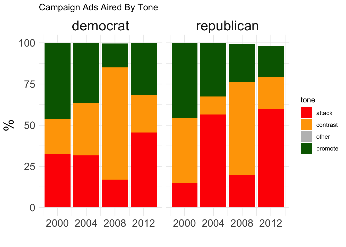
From above, we can see that Democratic campaigns had a roughly balanced distribution between attack, contrast, and promote ads in 2000 and 2004. Interestingly, there was a sharp increase in contrast ads in 2008, which immediately fell in 2012. Overall, we can see that promote ads (green) have generally decreased over time.
Similarly, Republican campaigns seemed to start with a higher proportion of promote ads in 2000, but have since noticeably declined in recent election cycles. Particularly in 2012, attack ads seem to dominate the Republican strategy.
When we think back to previous historic elections, the trends we’re observing make sense. In Bush vs Gore 2000, we observed Republicans use more promote ads, which tie to Bush’s “compassionate conservative” platform that focused on policy promotion. As we moved to 2004, the Iraq War and national security concerns began dominating election topics, fueling the fire behind attack ads.
Finally, the 2012 election revealed Romney’s dominant strategy with attack ads toward the incumbent, while Obama focused heavily on contrast ads that supplemented his distinguishing record and varying policies compared to Romney’s proposals.
To look more closely into these political ads, let’s understand the purpose behind them:
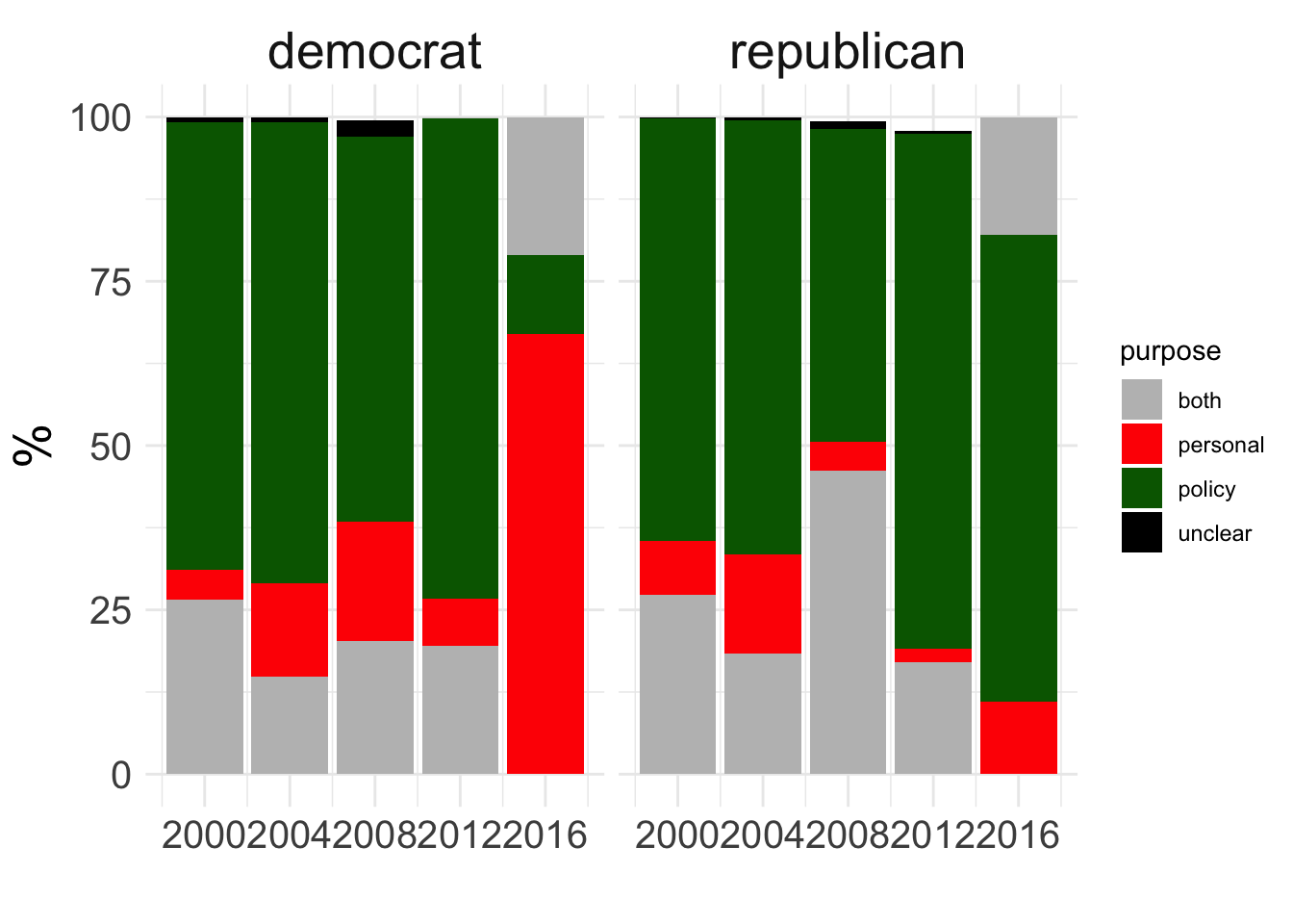
While most of the trends remain relatively consistent, 2016 represents an interesting case study. Here, we see that the Democratic Party significantly shifts towards personal ads, highlighting the increasing importance of personalization in modern politics and political campaigns. This can be especially effective as voter emotions have become heavily tied to a candidate’s character, leading to potential shifts in policy opinions, especially in an increasingly polarized political environment.
On the other hand, we can see how Republicans have consistently emphasized policy in their ad strategies, even in the contentious 2016 cycle. These include topics focused on tax reform, economic policy, immigration, national security, etc – which have been longstanding cornerstones of Republican platforms.
So Many Issues…
Now that we’ve understood the purpose and tone behind these campaign ads, and taken a glimpse at what these messages primarily focus on, let’s take a closer look at the top issues that these ads seem to highlight:
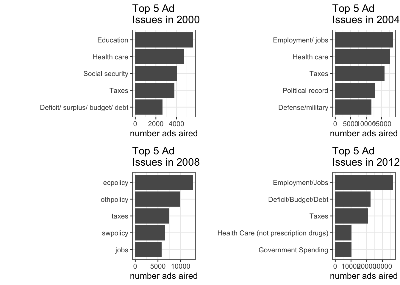
From the four plots, we can note some key overarching themes. First, we can see a notable shift from domestic issues (education, healthcare, and social security) to national security concerns from 2000 to 2004. Primarily due to 9/11, national security and defense emerge as key issues alongside ongoing economic concerns. The war on terror and foreign policy took center stage.
The next critical phase shift we see is the 2008 election during the financial crisis. Unsurprisingly, economic issues began dominating ads as candidates became focused on economic recovery, job creation, and stabilizing the financial system.
Overall, we can see how taxes and healthcare remain prominent across all years. This reflects ongoing debates about fiscal policy, government spending, and ultimately, the role of government in providing social services. Its consistency in multiple election cycles highlights how it has been a persistent issue for voters and candidates alike.
Case Studies
Let’s break down these themes further and examine the 2000 election in-depth:
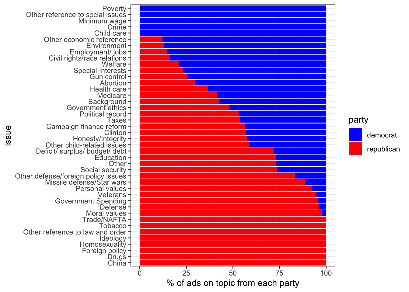
Here, we see a stark divide between the two parties’ focus areas. Democrats center on social justice, equality, welfare, and environmental protection, while Republicans emphasize more national security, foreign policy, military strength, and traditional social values.
Historically, the 2000 election between Bush and Gore was highly contentious, and the data above reflects each campaign’s strategy. Bush pushed for tax cuts, smaller government, and stronger defense. His focus on foreign policy is a reflection of the Republican desire to maintain US global leadership and military superiority.
Comparatively, Gore’s campaign focused on economic prosperity, environmental sustainability, and expanding social programs, which align with traditional Democratic priorities of governmental intervention to improve social welfare.
Now, let’s compare it to the 2012 election to see if things have shifted at all:
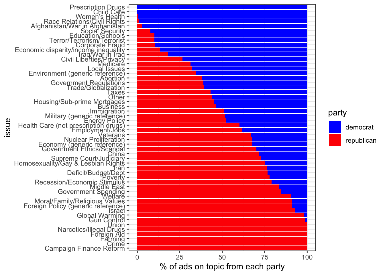
Here we can see that by 2012, the Democratic focus shifted more toward healthcare, women’s health, civil rights, and economic inequality. This highlights the Obama administration’s priorities, particularly with the defense of the Affordable Care Act and efforts to address income disparity in the wake of the financial crisis just several years prior.
Similarly, the Republican lens shifted towards more social issues like homosexuality, family values, and religious values, reflecting the increasing influence of socially conservative factions within the party.
Ultimately, we can observe a clear ideological divide between the two parties, which only widened in 2012. And, in the broader context of the 2008 financial crisis, both parties also adjusted their campaign ad strategies to emphasize economic issues.
Show Me The Money
Timing is everything in life. For campaign ads, it’s no different. Now that we’ve analyzed the trends behind the messages, let’s examine when the best time is to actually buy them:
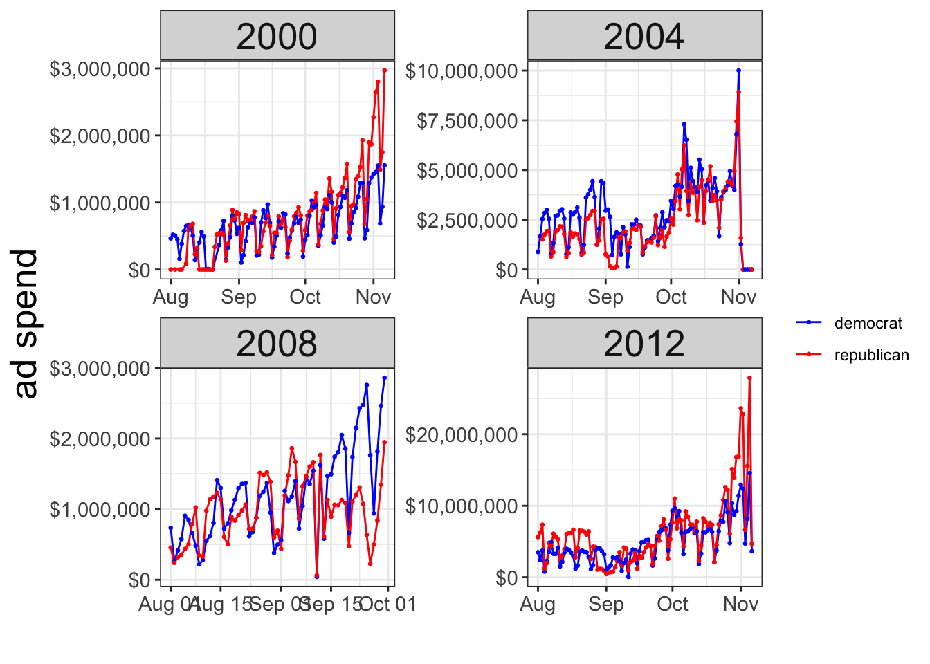
Overall, we see increased spending over time, with the most dramatic difference occurring between 2008 and 2012. Especially as digital and television ads become the primary way voters consume media, campaigns have adapted their spending strategies to capture voter attention.
More importantly, we see late-stage spending surges, particularly during the final days before November. This timing is key as it plays a critical role in last-minute voter persuasion, especially for undecided voters who are more likely to be swayed by media messages.
Outside spending and contributions have become a big part of campaigns since 2012, especially with the development of Super PACs, which can raise and spend nearly unlimited amounts of money to support or oppose specifically political candidates. As a result, both parties were able to spend far more on ads than in previous elections, leading to an unprecedented media surge, particularly in the final weeks of the campaign.
Facebook in 2020
As we’ve seen, social media has become a huge driver in terms of how candidates reach audiences and how voters consume campaign information and disinformation.
Let’s take a look at Biden’s Facebook ads in 2020 during the heat of the election:
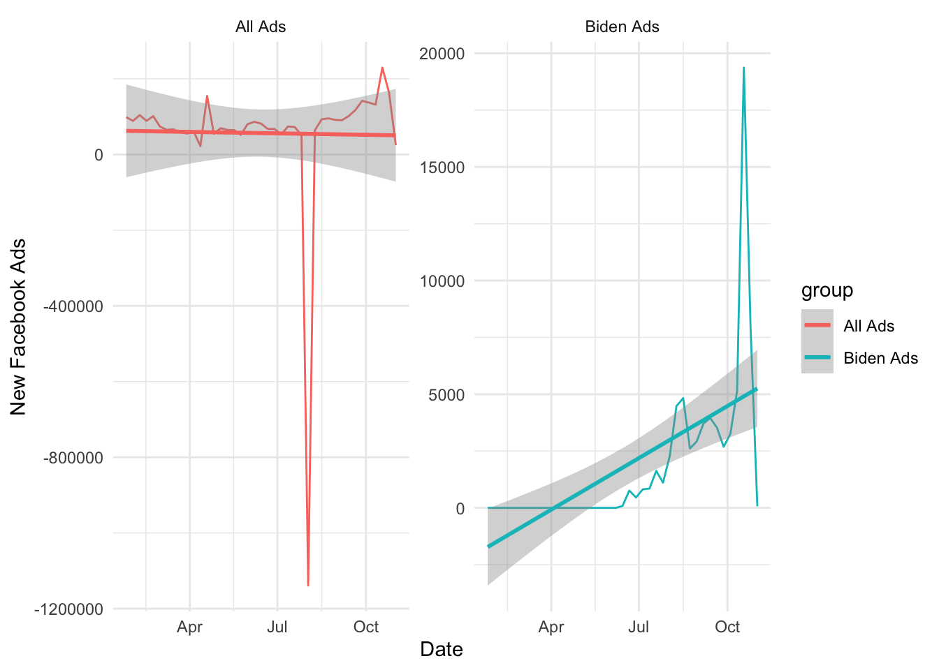
Overall, we can see a relatively stable pattern in the total number of new ads across all political campaigns. There seems to be a large drop, which could be due to data irregularities or reporting errors. After this, however, we observe a surge in the number of new ads leading up to the election, which confirms our previous analysis.
For Biden, we can see a steady increase throughout the campaign period, with its sharpest increase in October as the election nears.
Now, let’s dive into spending over time and see if we observe the same pattern:
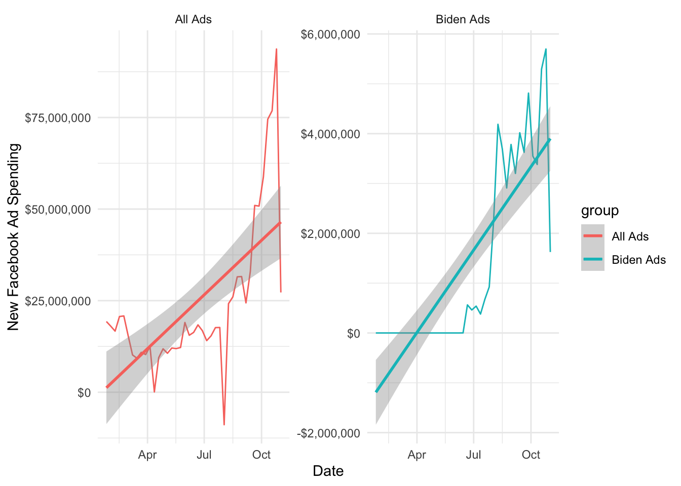
Aside from the data irregularity around August, the spending patterns appear to mirror that of the number of ads. Similarly, Biden’s ad spending also shows a general upward trend, with a sharp increase as the summer ends and the election date nears.
Bayesianism and Polls
As we saw in Blog Post 3, polling averages often reveal a lot about voters’ perceptions towards candidates. Here, we’ll apply Bayesian principles to consider prior beliefs based on historical trends and update them with new information, such as recent polling data, campaign spending, and other factors.
Under this methodology, we can see how campaigns may start with a strong belief about how certain states will vote, leading them to initially allocate fewer ad dollars to states where they feel confident based on historical trends (high prior). Thus, as new polling data comes in, more voter sentiment is revealed and campaigns begin shifting ad spending to influence state outcomes.
The late-stage ad surge we’re seeing reflects how campaigns are relying heavily on new polling information to strategize their final pushes and maximize influence on these state outcomes.
Let’s take a look at our model results:
##
## Call:
## lm(formula = D_pv2p ~ latest_pollav_DEM + mean_pollav_DEM + D_pv2p_lag1 +
##     D_pv2p_lag2, data = d.train)
##
## Residuals:
##      Min       1Q   Median       3Q      Max
## -12.2628  -2.4159  -0.3763   1.8844  14.4903
##
## Coefficients:
##                   Estimate Std. Error t value Pr(>|t|)
## (Intercept)        3.10835    0.98896   3.143  0.00177 **
## latest_pollav_DEM  0.82313    0.05720  14.389  < 2e-16 ***
## mean_pollav_DEM   -0.15327    0.04962  -3.089  0.00212 **
## D_pv2p_lag1        0.46877    0.02918  16.064  < 2e-16 ***
## D_pv2p_lag2       -0.13481    0.02632  -5.122 4.29e-07 ***
## ---
## Signif. codes:  0 '***' 0.001 '**' 0.01 '*' 0.05 '.' 0.1 ' ' 1
##
## Residual standard error: 3.784 on 511 degrees of freedom
## Multiple R-squared:  0.8333,	Adjusted R-squared:  0.832
## F-statistic: 638.5 on 4 and 511 DF,  p-value: < 2.2e-16
From above, we can see how latest_pollav_DEM is a strong predictor for the Democratic vote share, as every 1% increase in the latest polling average predicts a roughly 0.82% increase in Democratic vote share on average. In the context of Bayes, we see how the positive coefficient shows that new information from polling is a critical factor in updating prior beliefs.
However, the negative counterintuitive mean_pollav_DEM suggests that an increase in the mean polling average leads to a slight reduction in the Democratic vote share. This may be highlighting how candidates may peak early as an outlier to boost their mean polling average, while the latest polling is a more precise indicator.
Importantly, the Democratic vote share in the previous election is another strong predictor, which reflects the historical trend that voting patterns in states tend to be consistent across elections. In Bayesian terms, we have a strong prior belief that voting patterns are consistent.
Overall, the model has an R-squared value of 83% and a very low p-value, indicating quite a strong fit and statistically significant.
Let’s break it down even further and look at state-level analysis:
##             state year simp_pred_dem simp_pred_rep     winner stateab electors
## 1         Arizona 2024      52.37537      47.62463   Democrat      AZ       11
## 2      California 2024      65.50179      34.49821   Democrat      CA       54
## 3         Florida 2024      50.39256      49.60744   Democrat      FL       30
## 4         Georgia 2024      52.70412      47.29588   Democrat      GA       16
## 5        Michigan 2024      53.17941      46.82059   Democrat      MI       15
## 6       Minnesota 2024      55.45820      44.54180   Democrat      MN       10
## 7          Nevada 2024      52.73680      47.26320   Democrat      NV        6
## 8   New Hampshire 2024      55.53649      44.46351   Democrat      NH        4
## 9  North Carolina 2024      52.32944      47.67056   Democrat      NC       16
## 10           Ohio 2024      47.87625      52.12375 Republican      OH       17
## 11   Pennsylvania 2024      52.62631      47.37369   Democrat      PA       19
## 12          Texas 2024      49.66481      50.33519 Republican      TX       40
## 13       Virginia 2024      55.74610      44.25390   Democrat      VA       13
## 14      Wisconsin 2024      53.52559      46.47441   Democrat      WI       10
## 15       New York 2024      54.94712      45.05288   Democrat      NY       28
By looking at the simp_pred_dem values, we can immediately identify the swing states and solid democratic states. For the swing states like Florida, North Carolina, and Ohio, the democratic vote share seems to be highly contested, reflecting the competitive and battleground nature of these places.
Comparatively, the solid states have been won historically by the Democratic party, and with most of them having a large number of electoral college votes, this makes them even more crucial for a victory.
Let’s look at the final win predictions:
##             state year simp_pred_dem simp_pred_rep   winner stateab electors
## 1         Arizona 2024      52.37537      47.62463 Democrat      AZ       11
## 2      California 2024      65.50179      34.49821 Democrat      CA       54
## 3         Florida 2024      50.39256      49.60744 Democrat      FL       30
## 4         Georgia 2024      52.70412      47.29588 Democrat      GA       16
## 5        Michigan 2024      53.17941      46.82059 Democrat      MI       15
## 6       Minnesota 2024      55.45820      44.54180 Democrat      MN       10
## 7          Nevada 2024      52.73680      47.26320 Democrat      NV        6
## 8   New Hampshire 2024      55.53649      44.46351 Democrat      NH        4
## 9  North Carolina 2024      52.32944      47.67056 Democrat      NC       16
## 10   Pennsylvania 2024      52.62631      47.37369 Democrat      PA       19
## 11       Virginia 2024      55.74610      44.25390 Democrat      VA       13
## 12      Wisconsin 2024      53.52559      46.47441 Democrat      WI       10
## 13       New York 2024      54.94712      45.05288 Democrat      NY       28
##   state year simp_pred_dem simp_pred_rep     winner stateab electors
## 1  Ohio 2024      47.87625      52.12375 Republican      OH       17
## 2 Texas 2024      49.66481      50.33519 Republican      TX       40
## # A tibble: 2 × 3
##   winner         n    ec
##   <chr>      <int> <dbl>
## 1 Democrat      13   232
## 2 Republican     2    57
Overall, we can see that Democrats are in a strong position to win the election, with significant leads in many states. However, Republicans are still competitive as they have 57 EC votes from just 2 states, underscoring the importance of large and historically red states.
However, we also need to remember that the sample we’re seeing here is incomplete, and without predictions for key states like Pennsylvania, Michigan, or Wisconsin, it’s still hard to make a full determination of either party’s path to 270.
Repeated Bayes
To enhance our previous analysis, let’s preform repeated sampling of the test dataset to figure out what the average number won by Democrats and Republicans. This way, we can develop a more complete understanding of the average wins.
Let’s take a look:
## # A tibble: 2 × 4
##   winner     mean_states_won lower_ci_states upper_ci_states
##   <chr>                <dbl>           <dbl>           <dbl>
## 1 Democrat              8.36               6              11
## 2 Republican            1.45               1               2
Here, we can see that the Democrats are predicted to win roughly 8.36 states on average, with a confidence interval ranging from 6 to 11 states. This matches our previous analysis and highlights how Democrats are likely to secure a significant number out of the test dataset.
The Republican confidence interval is fairly narrow, indicating that the predictions are pretty consistent across the simulations. As a result, we’re seeing that based on the test dataset, the Republicans are struggling to gain ground based on historical polling data and previous election results. Of course, we need to consider possible limitations and how the test dataset may not fully capture the unexpected shifts in voter sentiment or last-minute changes that fuel surges in campaign spending.
With less than 3 weeks to go, it’s still anyone’s game. Stay tuned for more!
Data Sources:
Data are from the GOV 1347 course materials. All files can be found here. All external sources are hyperlinked.