This blog is an ongoing assignment for Gov 1347: Election Analytics, a course at Harvard College taught by Professor Ryan Enos. It will be updated weekly and culminate in a predictive model of the 2024 presidential election.
Introduction – What role does the VEP play in state-level election results? How effective is the ground game at swinging election outcomes? Ultimately, can campaign events help predict these results?
Knock knock. You open your front door to find a campaign volunteer, clipboard in hand, eager to talk to you about the upcoming election. We’ve all seen these people randomly roaming our neighborhoods. In reality, this is just one piece of the larger ground game strategy, where candidates and their teams hit the pavement, host rallies, and knock on doors to sway voters face-to-face. But with digital ads and viral tweets dominating the outreach scene, how effective is this old-school approach?
Some argue that this holds the secret to electoral success, while others say that rallies and door-knocking are more symbolic than substantial. So, can these campaign events and personal interactions really move the needle and predict state-level results? Or, is this all just political theater?
As always, let’s start with the data!
Back To Polls?
To begin our analysis, let’s take a step back and first examine state-specific forecasts for Democratic and Republican vote shares based on polling data:
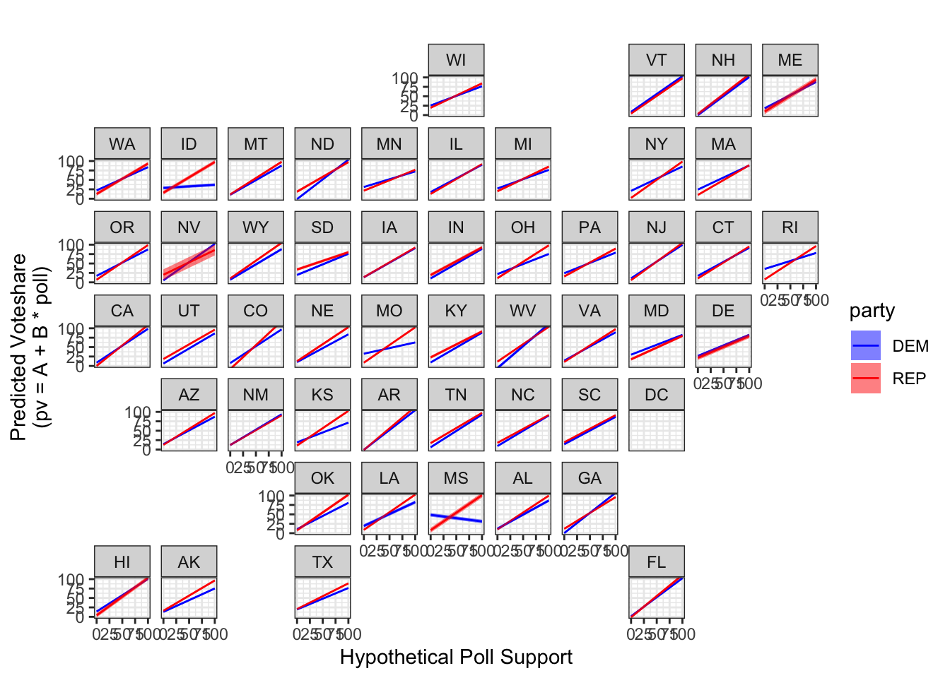
Here, we can see that for each state, the blue line represents the Democratic vote share prediction, while the red line represents the Republican vote share. Immediately, we notice that for most states, as poll support increases, the predicted vote share for both parties also increases. This makes sense.
However, there are also some issues with the plot. For example, some states have odd patterns, such as negative slopes or very high variance, suggesting that the linear models may not fit well in certain states. For example, in Nevada (NV), we see high variance in predictions, while in Mississippi (MS), there might be a negative slope, which is unrealistic for real-world elections. Historically, polling errors are more pronounced in states with smaller or harder-to-reach populations, such as Nevada. Other accuracy concerns include factors like partisan lean and polling methodology.
Thus, we’re seeing instances when polling data might be unreliable or where the relationship between polling support and actual vote share is rather weak.
Let’s take a closer look at two key states:
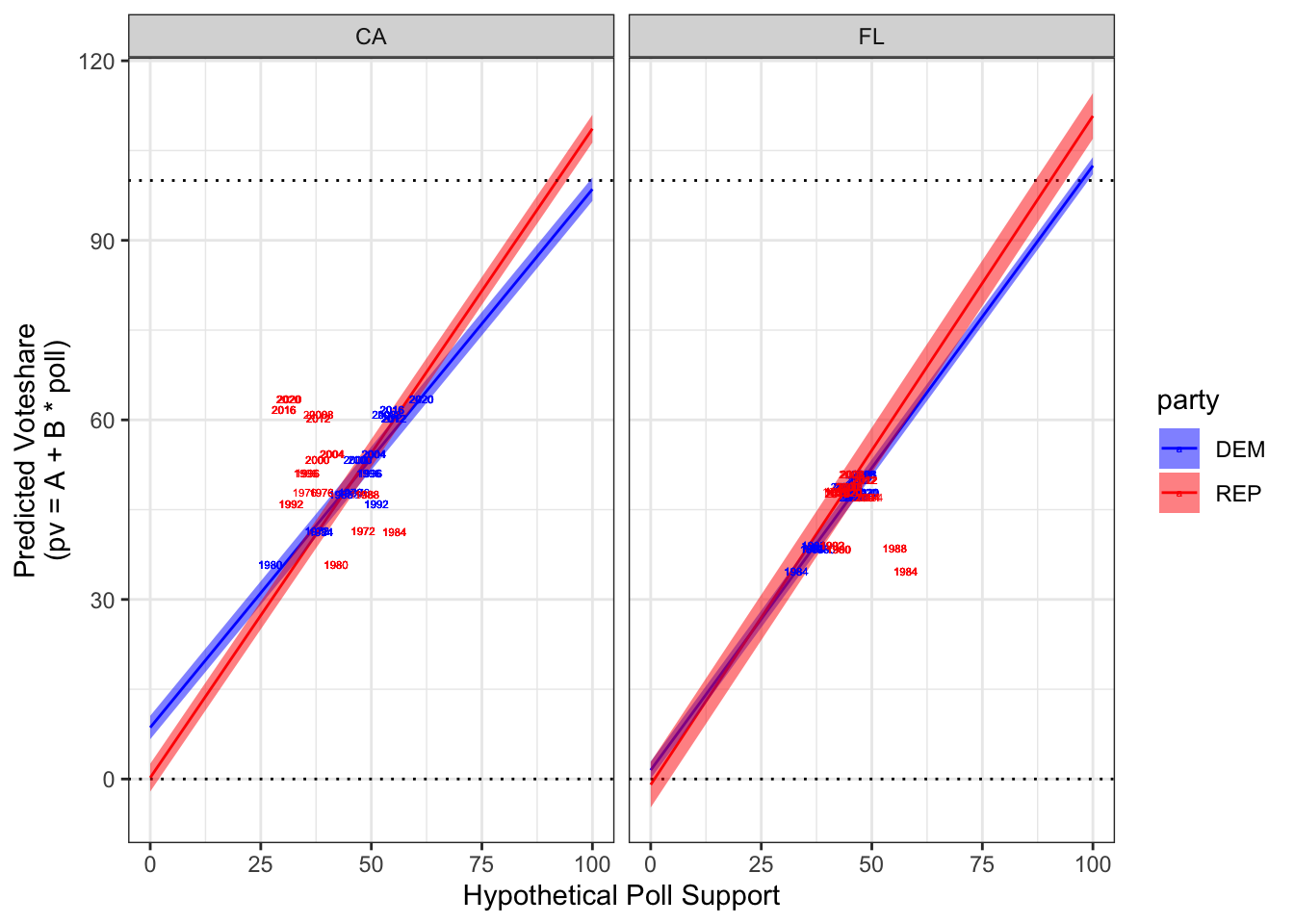
For California, we can see that the Democrats have a higher predicted vote share across almost all polling support levels compared to Republicans. Historically democratic years like 2020, 2016, and 2008 align closely with the predicted vote share for Democrats at mid-to-high polling support. On the other hand, years like 1980 and 1984 show Republicans doing better, but this makes sense as California was less reliably blue at the time.
In contrast, Florida reveals how the lines are closer together, indicating a more competitive electoral environment between the two parties. At the same time, the confidence intervals in Florida are wider, reflecting more uncertainty in the model’s predictions. This is likely due to Florida’s more volatile voting patterns and demographic shifts, making it harder to predict election outcomes based solely on polling.
Voting Eligible Population – Pennsylvania
Let’s take a deeper dive into the voting-eligible population (VEP). These people represent the portion of the population that is legally eligible to vote. Knowing the VEP helps in predicting election outcomes, especially in close races. A growing or shrinking VEP can significantly alter electoral dynamics, especially in battleground states.
Let’s examine a specific battleground case study:
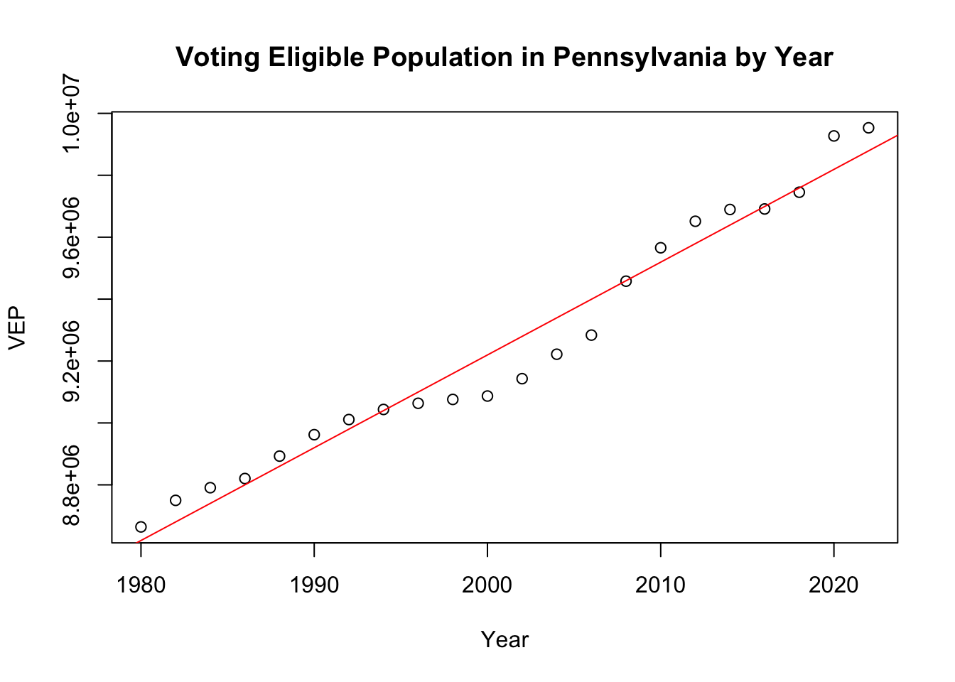
Here, we see that Pennsylvania has shown a steady, nearly linear increase in the VEP over the last few decades, reflecting population growth and demographic shifts. The red regression line hugs the points closely, predicting future VEP based on historical trends. Thus, we can ultimately assess how much influence a growing population could have on turnout rates and on election results.
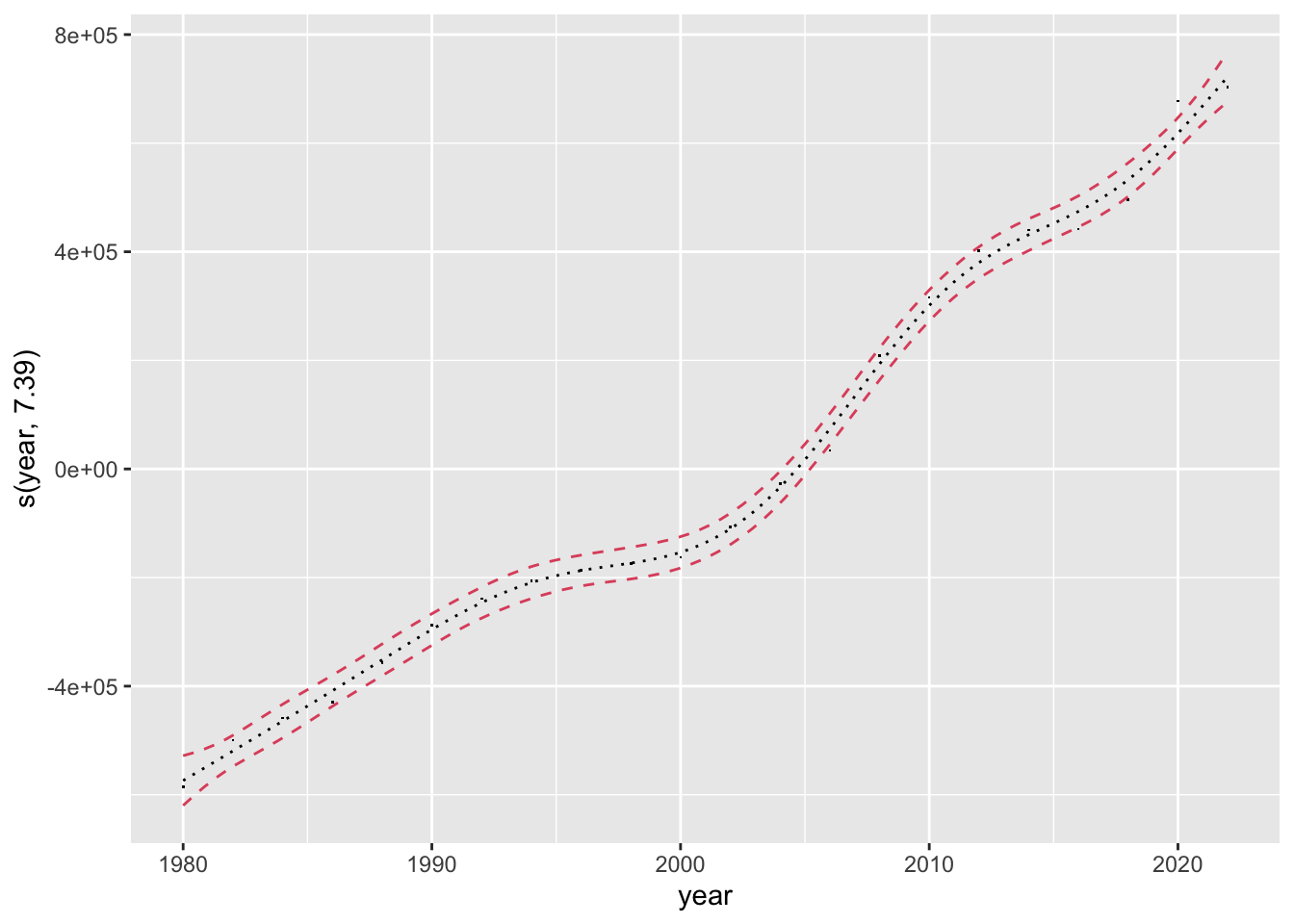
Now, let’s expand the OLS model to include generalized additive modeling (GAM) and use a weighted average to create a final prediction:
## [1] 10044706
Here, we’re adding a 75% weight to the GAM prediction, and a 25% weight to the OLS prediction. We can immediately see how GAM provides much more flexibility by allowing the model to fit a curved relationship between VEP and time, capturing complex demographic changes that might influence VEP growth in the future. As a result, our final VEP prediction for 2024 is approximately, 10,044,706.
Crossing 10 million eligible voters by the next election has significant implications for Pennsylvania’s electoral dynamics, as a larger electorate could change the composition of young voters, influencing overall turnout and election outcomes.
Field Offices and The Ground Game
Field offices play a crucial role in elections in terms of voter outreach and mobilization. These offices act as hubs for campaigns to connect directly with voters, organize events, and more. This allows for more specialized campaign strategies with tailored messaging and more rapid response to local issues.
Let’s trace the data across 2012 and 2016:
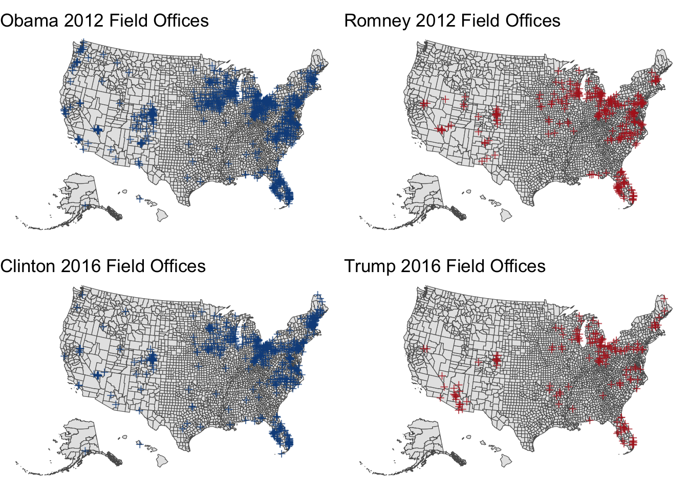
Here, we can see how the Obama campaign deployed a widespread and dense network of field offices, with a heavy concentration in battleground states like Ohio, Florida, and Pennsylvania. Clinton followed a similar strategy, with a focus on the Midwest battleground states. However, a lagging voter turnout in crucial areas especially among working-class voters in the Rust Belt was one of the reasons for her defeat.
The Republicans showed a significant shift from 2012 to 2016. We can see how Trump’s campaign had a more focused field office strategy, targeting specific battlegrounds like Florida, Pennsylvania, Ohio, and Michigan. However, his campaign relied heavily on digital outreach and rallies rather than a traditional field game. This unconventional method allowed him to increase his presence and reach, generating a high turnout, particularly in rural and exurban areas.
The Democratic Ground Game
Let’s dive deeper into Democratic field office work in battleground states by comparing some more historical trends:
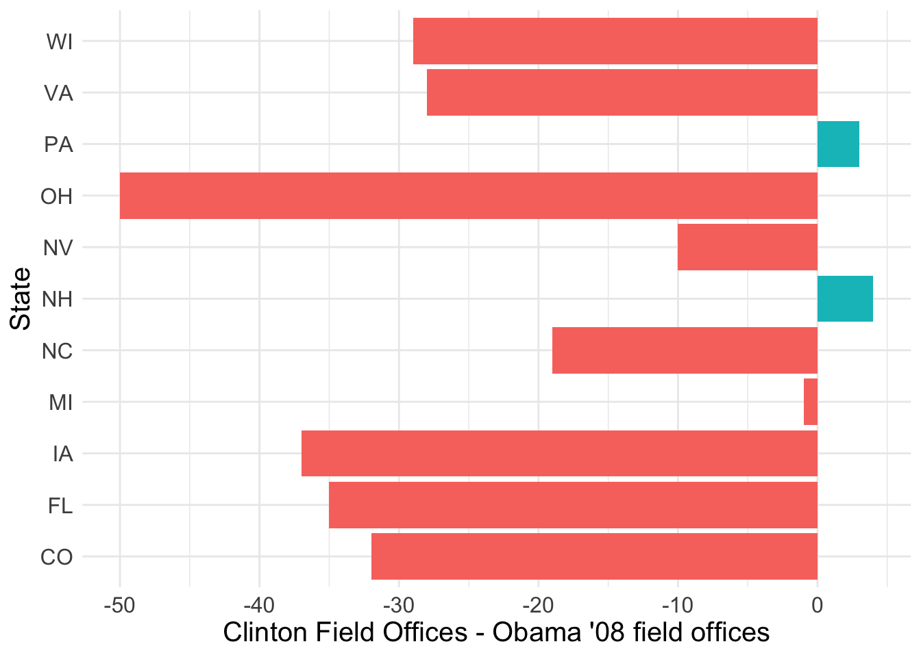
Here we can see how in most battleground states, Clinton had fewer field offices in 2016 than Obama did in 2008, indicated by the substantial negative values. This was detrimental when considering crucial states like Ohio, Florida, and Pennsylvania —- all critical swing states that contributed to Trump’s victory.
Ultimately, we see that the graph shows how Clinton’s campaign may have underinvested in field offices compared to Obama’s 2008 campaign, particularly in key Rust Belt states. These offices play a crucial role in get-out-the-vote (GOTV) efforts, volunteer mobilization, and localized campaign activities. This made it more challenging to mobilize Democratic voters, particularly in areas where voter enthusiasm may have been lower than in 2008.
Let’s continue our analysis by looking at 2012 and 2016:
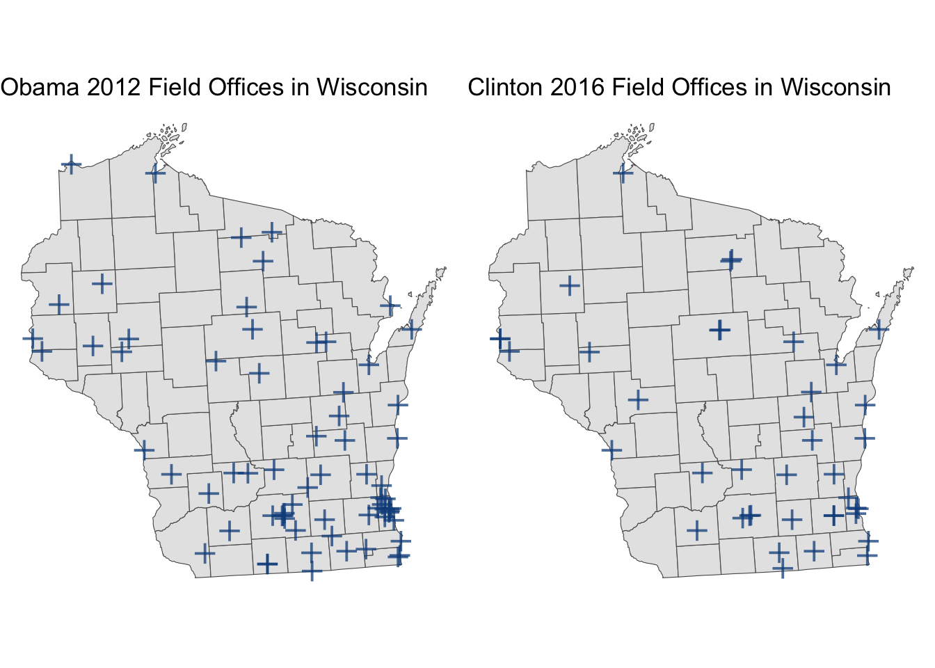
Once again, we see how Obama had a dense network of field offices spread across Wisconsin, particularly concentrated in urban and suburban areas, including the Milwaukee and Madison regions. His aggressive ground game aimed at reaching a wide range of voters through traditional canvassing and mobilization efforts. Comparatively, we can see Clinton’s fewer offices, especially in rural areas and northern parts of the state.
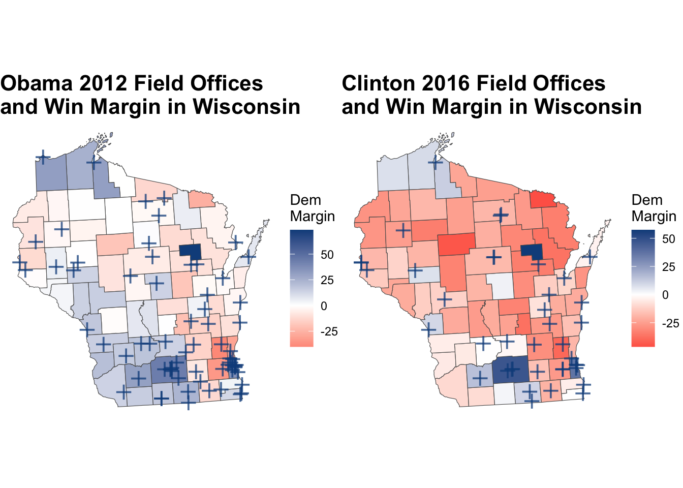
As expected, Obama won many counties by comfortable margins, particularly in urban areas like Milwaukee, Madison, and along the state’s southern border. His distribution across both urban and rural areas helped increase turnout in a wide range of regions.
Comparatively for Clinton, many of the counties turned red, highlighting how Trump outperformed Clinton in large parts of Wisconsin, especially in rural areas. Her concentrated efforts in urban areas came at the cost of losing support from rural and working-class voters.
So…What About 2024?
With the context and analysis we have now, let’s examine current trends and events:
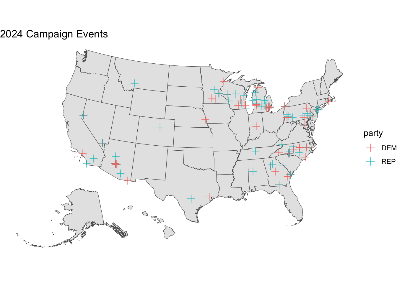
As predicted, both parties are concentrating their campaign events in battleground states like Michigan, Wisconsin, Pennsylvania, and Arizona. These are crucial Rust Belt states that helped decide the 2020 election results. They also have a significant presence in Georgia and Arizona, two historically Republican states that flipped to the Democrats in 2020, suggesting that Democrats are working to consolidate their gains in these areas.
The Republicans are also concentrating in battleground states, but are also hosting events in Ohio, Florida, and North Carolina, which have been traditionally red but occasionally competitive. Doing so will help secure support in historical strongholds while trying to gain a competitive edge in the swing states.
Overall, we can see how both parties are hosting fewer campaign events in traditionally solid states, allocating more of their resources to swing states where the outcomes are more unpredictable.
Campaign Events and Predicting Vote Share?
We can clearly see trends in campaign events, presence in battleground states, and historical results. Thus, can we use this information to improve our model and predict vote share?
Let’s find out:
##
## Call:
## lm(formula = D_pv2p ~ n_ev_D + ev_diff_D_R, data = d)
##
## Residuals:
##      Min       1Q   Median       3Q      Max
## -17.6200  -4.7648   0.3904   5.2448  16.4092
##
## Coefficients:
##             Estimate Std. Error t value Pr(>|t|)
## (Intercept) 48.18936    0.36910 130.559  < 2e-16 ***
## n_ev_D       0.12588    0.03351   3.757 0.000186 ***
## ev_diff_D_R  0.10453    0.06726   1.554 0.120618
## ---
## Signif. codes:  0 '***' 0.001 '**' 0.01 '*' 0.05 '.' 0.1 ' ' 1
##
## Residual standard error: 7.508 on 711 degrees of freedom
##   (6896 observations deleted due to missingness)
## Multiple R-squared:  0.02141,	Adjusted R-squared:  0.01866
## F-statistic: 7.778 on 2 and 711 DF,  p-value: 0.0004554
Here, we can see that for each additional Democratic event in a state, the Democratic vote share is expected to increase by roughly 0.126 percentage points, with a statistically significant p-value. However, the R-squared value is very low, suggesting that it only captures roughly 1.87% of the variance in state-level vote share based on the number of campaign events and the event difference.
Is this consistent with the Republican model?
##
## Call:
## lm(formula = R_pv2p ~ n_ev_R + ev_diff_R_D, data = d)
##
## Residuals:
##      Min       1Q   Median       3Q      Max
## -16.4088  -5.2449  -0.3903   4.7647  17.6204
##
## Coefficients:
##             Estimate Std. Error t value Pr(>|t|)
## (Intercept) 51.81023    0.36913 140.359  < 2e-16 ***
## n_ev_R      -0.12586    0.03351  -3.756 0.000187 ***
## ev_diff_R_D  0.23042    0.07796   2.956 0.003222 **
## ---
## Signif. codes:  0 '***' 0.001 '**' 0.01 '*' 0.05 '.' 0.1 ' ' 1
##
## Residual standard error: 7.509 on 711 degrees of freedom
##   (6896 observations deleted due to missingness)
## Multiple R-squared:  0.02141,	Adjusted R-squared:  0.01865
## F-statistic: 7.776 on 2 and 711 DF,  p-value: 0.0004564
Interestingly, the model predicts that for each additional Republican event, the Republican vote share decreases by roughly 0.126 percentage points, with a statistically significant p-value. This could mean that Republicans tend to hold events in more competitive or difficult states, where their baseline support is lower.
However, the positive association in ev_diff_R_D suggests that Republicans benefit more then they hold more events than Democrats, showing how the ground game is particularly effective when they out-campaign Democrats in terms of event presence.
Still, the very low R-squared value suggests that while campaign events can influence voter engagement and media coverage, they cannot account for most of the variance in state-level vote shares. Statistically, the high residual standard error compared to the effect sizes indicates that there is a lot of unexplained noise in the relationship between the predictors. While the coefficients are statistically significant, meaning there is some measurable impact on vote share, it is relatively small in the broader context of all factors that determine election outcomes that we’ve seen in previous blogs.
Thus, I predict that its addition to our model will likely produce negligible impact…especially when election day is only 14 days away!
Stay tuned!
Data Sources:
Data are from the GOV 1347 course materials. All files can be found here. All external sources are hyperlinked.