This blog is an ongoing assignment for Gov 1347: Election Analytics, a course at Harvard College taught by Professor Ryan Enos. It will be updated weekly and culminate in a predictive model of the 2024 presidential election.
So, the time has come…
After weeks of diving into the mechanics of elections – from economic trends to ground game tactics, from polling swings to those elusive “October surprises”, and even shark attacks – it’s finally time to put our analysis to the test. The big question on everyone’s mind is: what’s our prediction?
As we wrap up this journey, I think back to a classic saying that echoes through every stats class – “All models are wrong, but some are useful.”
In other words, no prediction tool is perfect, but with the right approach, we might just capture some meaningful insights. So, while no model can account for every quirk and curveball, I’m excited to share my final forecast for this election. Maybe it’s right. Maybe not.
Regardless, let’s dive in and see what our analysis reveals!
The Final Model
In our previous blog, we discussed not only the influence of shocks but also decided on a final model we would use. This model hinges on ANES data, economic factors, and random forest computation to produce its results.
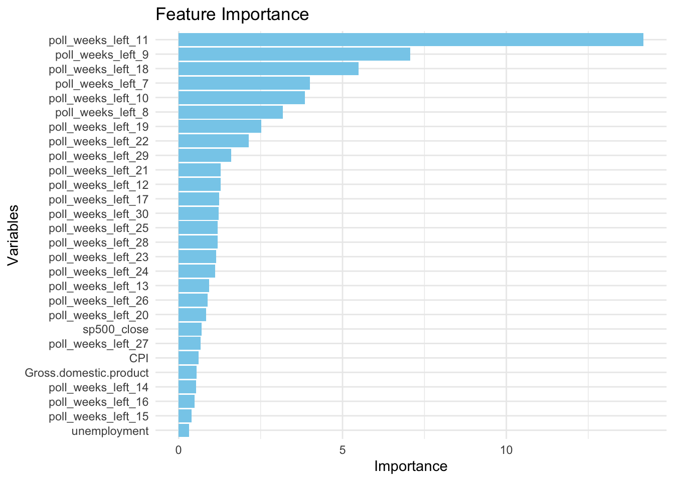
Before we dig in, let’s take a look at the feature importance:

Interestingly, we can see how the random forest model is relying heavily on polling data, which can be positive as it reveals recent voter sentiment, but also may not fully capture economic shocks. However, by weighting polling data heavily, the model is well-suited for situations where the electorate’s final preferences align with polling trends. Further, while economic factors have lower importance, the model is still considering its background influence, providing a baseline for voter sentiment.
Throughout my research and investigation, I’ve found that voter sentiment and economic well-being significantly impact how voters feel about the incumbent party and potential candidates. When the economy is doing well, voters tend to feel more secure and may attribute positive economic outcomes to the current administration or the incumbent party. On the other hand, economic downturns or periods of high unemployment can lead to dissatisfaction with the incumbent and voters looking for change.
More broadly, we can see this central idea in political science as the retrospective voting theory, suggesting that voters make decisions based on the past performance of a candidate or party – economic conditions are just one measure of this performance.
Historically, we’ve seen this phenomenon play out. In the 1980 election between Carter and Reagan, we saw how high inflation and unemployment caused voters to be frustrated with President Carter, contributing to a landslide victory for Reagan.
Similarly, the 1992 election between Bush and Clinton saw the catchphrase “It’s the economy, stupid” as the central statement for Clinton’s campaign, highlighting the recession that affected Bush’s approval. In particular, economic factors like unemployment and GDP growth were especially divisive, leading voters to seek an alternative candidate.
Ultimately, by combining ANES data with economic indicators, the model can account for both personal factors (such as demographics and political attitudes) and external, quantifiable economic conditions that influence elections and voter sentiment.
And so, let’s take a look at the 2024 prediction results before further analysis and investigation:
## Predicted Vote Shares for 2024 Election:
## Democratic candidate (Harris): 52.88 %
## Republican candidate (Trump): 47.72 %
Here, we can see how Harris leads with a small advantages, but the estimates still imply a fairly narrow margin, highlighting the competitiveness of this presidential race. The small increase in predicted vote share for Harris compared to previous models makes sense as economic data like GDP, unemployment rate, CPI, and the S&P favor the incumbent party when the economy is doing well.
To further investigate our model, I conducted a cross-validation test that produced surprising results:
## Random Forest
##
## 448 samples
##  28 predictor
##
## No pre-processing
## Resampling: Cross-Validated (10 fold)
## Summary of sample sizes: 404, 404, 402, 403, 402, 404, ...
## Resampling results:
##
##   RMSE         Rsquared   MAE
##   0.003043932  0.9999996  0.0009377337
##
## Tuning parameter 'mtry' was held constant at a value of 9
## Tuning
##  parameter 'splitrule' was held constant at a value of variance
##
## Tuning parameter 'min.node.size' was held constant at a value of 5
## [1] "Cross-validated RMSE: 0.00304393235350963"
## [1] "Cross-validated R-squared: 0.999999560925517"
Interestingly, we can see an R-squared value of nearly 1, suggesting that the model has a near-perfect explanatory power over the training data. However, this indicates potential overfitting and whether the model is simply capturing the “noise” of the dataset.
Thus, my next steps will be to ensure its reliability by conducting in-sample, out-sample of sample, and bootstrapped prediction estimates to further evaluate the precision of my model.
Let’s dive in!
In-Sample and Out-of-Sample Tests
We’ll start with an in-sample test, whereby the model is evaluated on the same data it was trained on, which usually produces lower error but may not reflect the true predictive power on new data:
## In-Sample RMSE: 0.0006174325
Here, we can see that an extremely low RMSE means that the model fits the training data extremely well, but also means that there is some potential overfitting. This happens when the model is adjusted too precisely to historical patterns, which may not hold for future data.
Let’s see if this remains true for an out-of-sample test, in which the model is evaluated on data it hasn’t seen, such as holding out certain data points to provide a better assessment of how it might perform on new data:
## Training RMSE (excluding 2008 and 2012): 0.0006013352
## Pseudo-Test RMSE (2008 and 2012): 2.430502
I chose not to test the model on the two most recent elections (2016 and 2020) due to the presence of unique factors. In particular, the political polarization of 2016 and the global pandemic in 2020 heavily influenced the election environment, which may suggest that the model does more poorly than in reality.
Regardless, we can see the large difference between the Training RMSE and the Pseudo-Test RMSE, highlighting the model’s high accuracy on the training set but its inability to handle variations in real-world election conditions. At the same time, the 2008 and 2012 elections posed interesting factors, with Barack Obama as the first African American presidential nominee for a major party in 2008 and the 2012 election with the 2008 financial crisis still in its rearview mirror.
Thus, the model may not be flexible enough to account for these unusual election dynamics, which could explain the high error.
Let’s repeat our analysis to generate a prediction interval:
The Predictive Interval
## Predicted Vote Share for 2024:
## Mean Prediction: 52.81 %
## 95% Prediction Interval: 52.77 % to 52.85 %
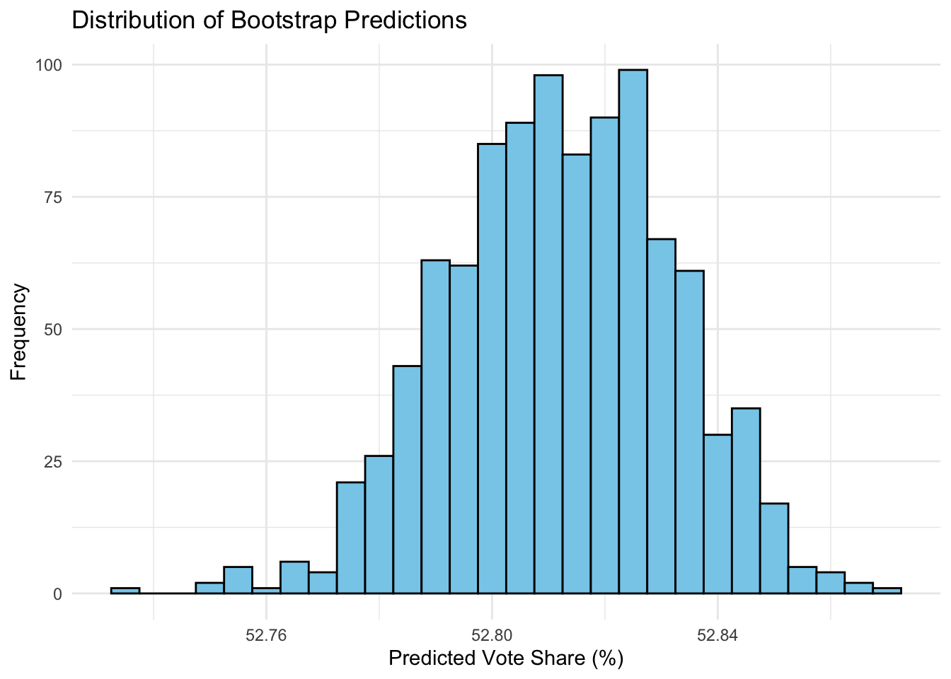
The 95% prediction interval is extremely narrow, spanning only 0.08 percentage points (from 52.77% to 52.85%). Thus, this suggests that there is very little variability in the model’s predicted outcomes. At the same time, we need to consider potential overconfidence and how election outcomes often vary due to last-minute shifts in voter sentiment and unpredictable factors.
As we’ve seen before, there are potential questions about overfitting, and so the lack of flexibility in the model could mean that it is highly deterministic, focusing heavily on a few key predictors.
We can also visualize these replications in a histogram:

Ultimately, the narrow 95% prediction interval suggests strong confidence in this specific outcome, but may not fully account for real-world uncertainties and sudden shifts that characterize, or perhaps plague, elections.
Now We Wait…
With election night just 24 hours away, the world sits on the edge of their seats (or perhaps their couches), anxiously awaiting the results. I know I’ll be glued to the TV.
For weeks, we’ve uncovered the dynamics of this election – from the economic climate to voter sentiment, from polls to historical trends. Yet, even with the most advanced model at our fingertips, one thing remains certain – elections are full of surprises.
Either way, this process reminds us of the power and limits of data-driven insights. Ultimately, every vote and every voice counts. So, now we wait…
Data Sources:
Data are from the GOV 1347 course materials. All files can be found here. All external sources are hyperlinked.